Machine Learning
Machine Learning is the art of programming computers so they can learn from data.
In practice, ML is mostly done in Python and tasks usually involve
- Scikit-Learn which has a large collection of canned algorithms (start here),
- TensorFlow for deep learning
Scikit-Learn ML Map
 Periodic Table of ML
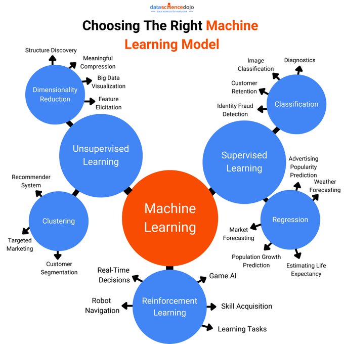
ML algorithms can be grouped into these categories:
The data may arrive 2 different ways.
- In Batch Learning, the system is trained using all available data.
- In Online Learning, the system is trained incrementally by feeding it data in mini-batches.
The algorithm may generalize in 2 different ways.
- In Instance-Based Learning, the system learns examples by rote, then generalizes to new cases using a similarity measure.
- In Model-Based Learning, a model is built from a set of examples, then the model is used to make predictions.
Model training can go wrong in several ways. ML Challenges
Feature engineering involves feature selection, feature extraction and feature creation.
To train the model, data is divided into ML Data Sets.
As a general rule, the project will follow a pretty standard ML Workflow.
A binary classifier distinguishes between 2 classes.
cross_val_score() splits the dataset into K-folds, then evaluates predictions made on each using a model trained on the remaining folds.
cross_val_predict() gets the actual predictions of the K-folds.
confusion_matrix() creates a matrix of true and false predictions, with true values on the diagonal.
precision = TP / (TP + FP)
recall (a.k.a sensitivity, true positive rate) = TP / (TP + FN)
F₁ = TP / (TP + (FN + FP)/2)
precision_recall_curve() computes precision and recall for all possible threasholds.
Another way to select a good precision/recall tradeoff is to plot precision vs. recall.
ROC = receiver operating characteristic
TPR = true positive rate (= recall)
TNR = true negative rate (= specificity)
FPR, FNR = false positive rate, false negative rate
An ROC curve plots sensitivity (recall) vs. 1 - specificity.
roc_curve() computes the ROC curve.
A good ROC AUC (area under curve) has a value close to 1, whereas a random classifier has a value of 0.5
roc_auc_score() computes the ROC AUC.
OvO = one vs. one
OvA = one vs. all, one vs. rest
Multilabel classification outputs multiple binary labels.
Multioutput classification output multiple multiclass labels.
Linear regression model prediction
Vectorized form
Cost function of the linear regression model
Normal equation
MSE for a linear regression model is a convex function, meaning that a line segment connecting any 2 points on the curve never crosses the curve. This implies there are no local minima, just one global minimum.
Preprocess the data with Scikit-Learn’s StandardScalar
Batch Gradient Descent
Partial derivatives of the cost function
Gradient vector of the cost function
$$\nabla_\theta MSE(\theta)=\begin{pmatrix} \frac{\delta}{\delta\theta_0}MSE(\theta) \ \frac{\delta}{\delta\theta_1}MSE(\theta) \ \vdots \ \frac{\delta}{\delta\theta_n}MSE(\theta) \end{pmatrix} =\frac{2}{m}\textbf{X}^T\cdot(\textbf{X}\cdot\theta-\textbf{y})$$
Gradient descent step
Stochastic Gradient Descent
Regularized Linear Models
- Ridge regression adds a regularization term to the cost function, forcing the learning algorithm to keep the weights as small as possible.
- Lasso regression tends to completely eliminate the weights of the least important features.
- Elastic Net is a combination of the two.
- Early stopping
Logistic regression
estimates the probability that an instance belongs to a particular class.
The logistic regression loss function is convex
and its derivative is
To train a logistic regression model
Softmax Regression / Multinomial Logistic Regression
Softmax score for class k
Softmax function
Softmax prediction
Cross entropy cost function
Cross entropy gradient vector
Support Vector Machines
Support vectors are data instances on the “fog lines” of the decision boundary “street”.
Soft margin classification allows some margin violations, controlled by the C parameter.
Nonlinear SVM Classification
The SVC class implements the kernel trick, whatever that is, which runs higher degree polynomial efficiently.
Gaussian radial bias function (RBF)
Increasing gamma makes the bell-shape curve narrower.
SVM Regression
SVMs also support linear and nonlinear regression.
Decision Trees
A decision tree is a white box model that can be visualized.
Decision tree prediction
Regularization hyperparameters
max_depthmin_samples_splitmin_samples_leafmin_weight_fraction_leafmax_leaf_nodesmax_features
Regression Trees
Weaknesses of decision trees
- Sensitive to orientation of training data. PCA can help.
- Sensitive to small variations of training data.
Ensemble Methods
An ensemble can be a strong learner even if each classifier is a weak learner, if there are enough of them and they are diverse enough.
A hard voting classifier predicts the class that gets the most votes.
A soft voting classifier makes predictions based on the averages of class probabilities.
Bagging (bootstrap aggregating) is training classifiers on different subsets of data with replacement.
Pasting is the same thing without replacement.
Random patches sample both training instances and features.
A random forest is an ensemble of decision trees.
The ExtraTreesClassifier (extra = extremely randomized) uses random thresholds for each feature and has higher bias & lower variance than the RandomForestClassifier.
The RandomForestClassifier has a feature_importances_ variable which is handy for selecting features.
Boosting
Boosting (hypothesis boosting) combines weak learners into a strong learner by training learners sequentially.
AdaBoost (adaptive boosting) trains each learner on instances that its predecessor underfitted.
Gradient boosting tries to fit the new predictor to the residual errors made by the previous predictor.
Stacking (stacked generalization)
Stacking trains a model to make a final prediction, instead of hard or soft voting.
The final predictor is called a blender.
The blender is typically trained on a hold-out data set.
Dimensionality Reduction
Principle Component Analysis (PCA) identifies the hyperplane that lies closest to the data, then projects the data onto it.
The principle components can then be accessed with the components_ variable. Also interesting is the explained_variance_ratio_ variable.
To find the minimum components to preserve a given variance, use
Reconstruct the original set with
PCA loads the entire dataset into memory. For large datasets, use Incremental PCA.
When d is much smaller than n, randomized PCA can give much faster results.
Kernel PCA
Other
- Locally Linear Embedding (LLE) is a manifold learning technique that looks at how each instance relates to its neighbors, then tries to preserve the relationship in lower dimensions.
- Multidimensional Scaling (MDS) attempts to preserve the distances between instances
- Isomap creates a graph between instances, then reduces dimensionality while trying to preserve geodesic distances between instances
- t-Distributed Stochastic Neighbor Embedding (t-SNE) reduces dimensionality while keeping similar instances together and dissimilar instances apart. Used mostly for visualization.
- Linear discriminant analysis (LDA) is a classifier that learns the most discriminative axes between the classes.